
by Steve Knudtsen
Abstract
LTspice® can be used to perform statistical tolerance analysis for complex circuits. This article will present techniques for tolerance analysis using Monte Carlo and Gaussian distributions and worst-case analysis within LTspice. To show the efficacy of the method, a voltage regulation example circuit is modeled in LTspice demonstrating Monte Carlo and Gaussian distribution techniques for the internal voltage reference and feedback resistors. The results of this simulation are compared to a worst-case analysis simulation. Included are four appendices. Appendix A provides insights on the distribution of trimmed voltage references. Appendix B provides an analysis of the Gaussian distribution in LTspice. Appendix C provides a graphical view of the Monte Carlo distribution as defined by LTspice. Appendix D provides instructions for editing LTspice schematics and extracting the simulated data.
This article illustrates statistical analysis that can be done with LTspice. This is not a review of 6-sigma design principles, the central limit theorem, or Monte Carlo sampling.
Tolerance Analysis
In system design, parametric tolerance constraints must be considered to ensure a successful design. A common approach uses worst-case analysis (WCA) where all parameters are adjusted to their maximum tolerance limit. In a worst-case analysis, the performance of the system is analyzed to determine if the worst-case result lies within the system design specification. There are limitations to the efficacy of WCA such as:
• WCA requires determining which parameters must be maximized or minimized for a true worst-case result.
• WCA results often violate design specification requirements, leading to expensive component selection to obtain acceptable results.
• WCA results statistically do not represent commonly observed results; to observe a system exhibiting WCA performance may require a very large number of assembled systems.
An alternate approach for system tolerance analysis is to use statistical tools for component tolerance analysis. The benefit of a statistical analysis is the resulting data has a distribution that reflects what should be commonly measured in physical systems. In this article, LTspice is used to simulate circuit performance with Monte Carlo and Gaussian distributions applied to parametric tolerance variation. This is compared to a WCA simulation.
Despite the noted issues with WCA, both worst-case and statistical analysis provide valuable insights to system design. For a very helpful tutorial on applying WCA using LTspice, please see “LTspice: Worst-Case Circuit Analysis with Minimal Simulations Runs” by Gabino Alonso and Joseph Spencer.
Monte Carlo Distribution
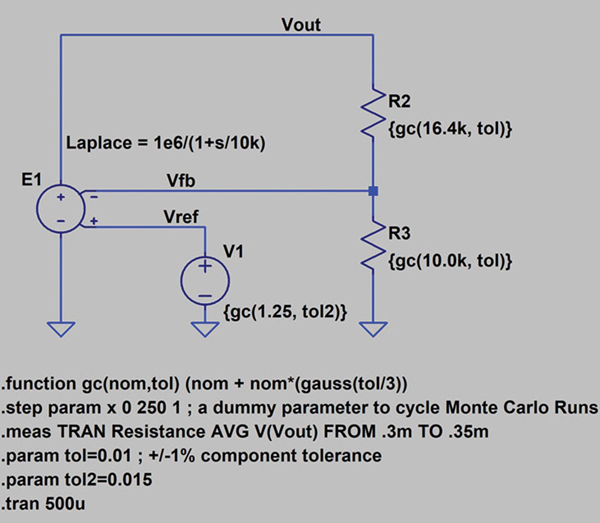
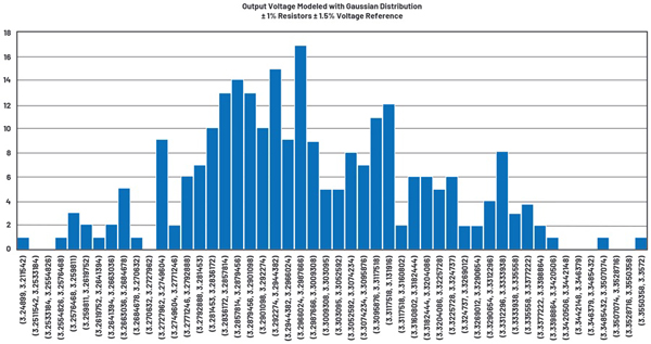
Figure 1 shows a voltage reference modeled in LTspice with a Monte Carlo distribution. The voltage source is nominally 1.25 V, and the tolerance is 1.5%. The Monte Carlo distribution defines 251 voltage states within the 1.5% tolerance range. Figure 2 shows the histogram of the 251 values with 50 bins. Table 1 illustrates the associated statistics of the distribution.
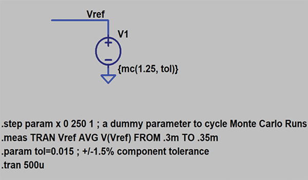
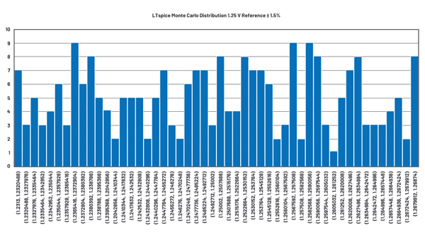
Table 1. Statistical Analysis of Monte Carlo Simulation Results
| Result | |
| Average | 1.249933 |
| Minimum | 1.2313 |
| Maximum | 1.26874 |
| Standard Deviation | 0.010615 |
| Error Positive | 1.014992 |
| Error Negative | 0.98504 |
Gaussian Distribution
Figure 3 shows a voltage reference modeled in LTspice with a Gaussian distribution. The voltage source is nominally 1.25 V, and the tolerance is 1.5%. The Monte Carlo distribution defines 251 voltage states within the 1.5% tolerance range. Figure 4 shows the histogram of the 251 values with 50 bins. Table 2 illustrates the associated statistics of the distribution.
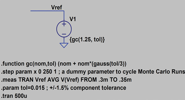
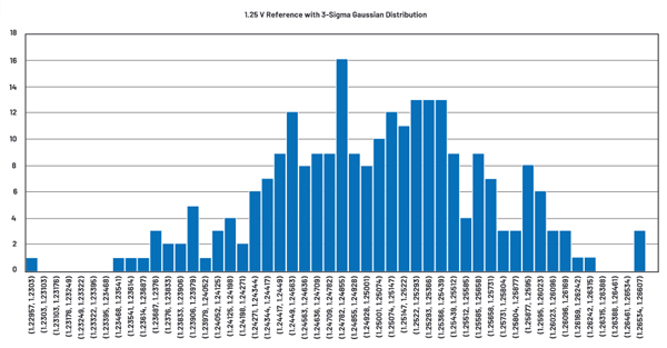
Table 2. Statistical Analysis of Gaussian Reference Simulation Results
| Result | |
| Minimum | 1.22957 |
| Maximum | 1.26607 |
| Average | 1.25021 |
| Standard Deviation | 0.006215 |
| Error Positive | 1.012856 |
| Error Negative | 0.983656 |
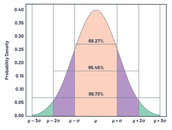
Gaussian distributions are normal distributions with a bell-shaped curve and the probability density shown in Figure 5.
The correlation between ideal and LTspice simulated Gaussian distributions is shown in Table 3.
Table 3. Statistical Distribution of 251-Point LTspice Simulated Gaussian Distribution
| Simulated | Ideal | |
| 1-Sigma Spread | 67.73% | 68.27% |
| 2-Sigma Spread | 95.62% | 95.45% |
| 3-Sigma Spread | 99.60% | 99.73% |
To summarize the above simulations, LTspice can be used to simulate a Gaussian or Monte Carlo tolerance distribution for a voltage source. This voltage source can be used to model a reference in a DC-to-DC converter. The LTspice Gaussian distribution simulation matches closely with the predicted probability density distribution.
Tolerance Analysis for DC-to-DC Converter Simulation
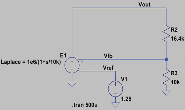
Figure 6 is an LTspice simulation schematic for a DC-to-DC converter using a voltage controlled voltage source to model closed-loop voltage feedback. The feedback resistors R2 and R3 are nominally 16.4 kΩ and 10 kΩ. The internal voltage reference is nominally 1.25 V. In this circuit, the nominal regulated voltage, VOUT, or setpoint is 3.3 V.
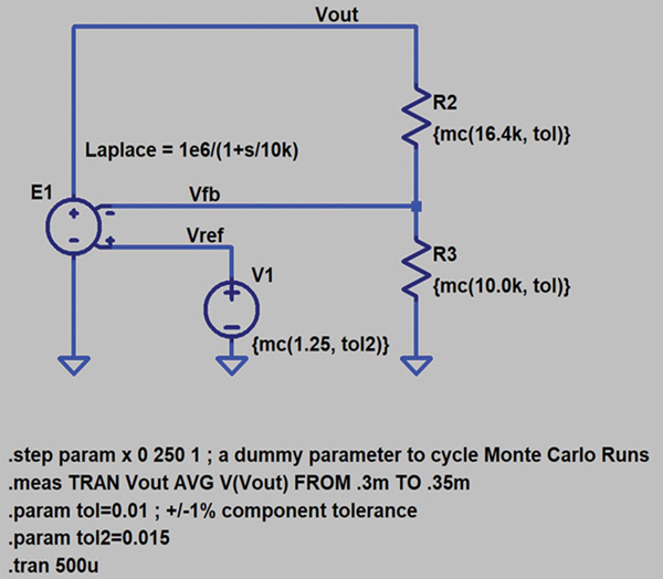
To simulate the tolerance analysis of voltage regulation, feedback resistors R2 and R3 are defined with a tolerance of 1%, and the internal voltage reference is defined with a tolerance of 1.5%. Three methods for tolerance analysis will be presented in this section: statistical analysis using a Monte Carlo distribution, statistical analysis using a Gaussian distribution, and a worst-case analysis (WCA).
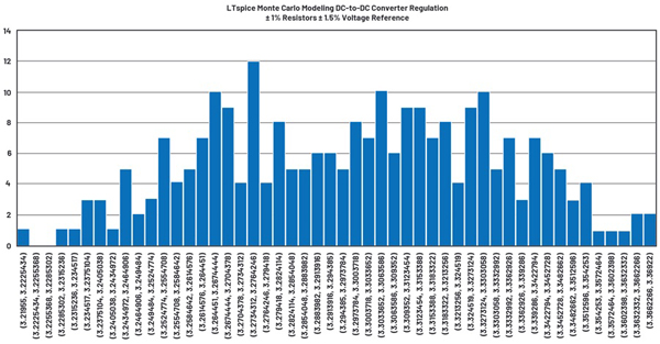
Figures 7 and 8 illustrate the schematic and voltage regulation histogram for a simulation using Monte Carlo distributions.
Figures 9 and 10 illustrate the schematic and voltage regulation histogram for a simulation using Gaussian distributions.
Figures 11 and 12 illustrate the schematic and voltage regulation histogram for a simulation using WCA.
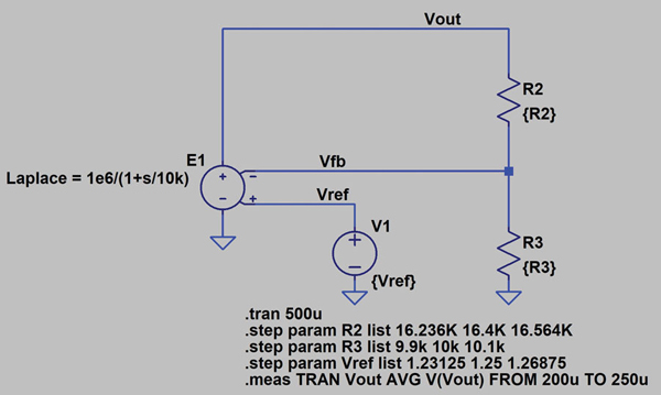
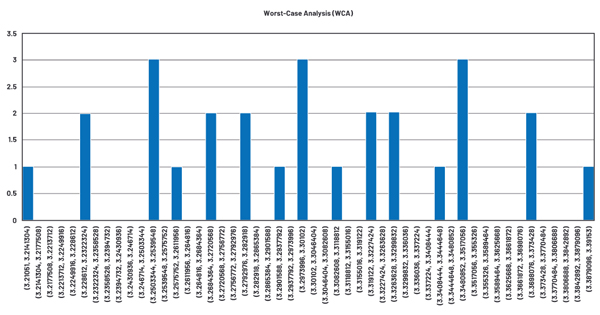
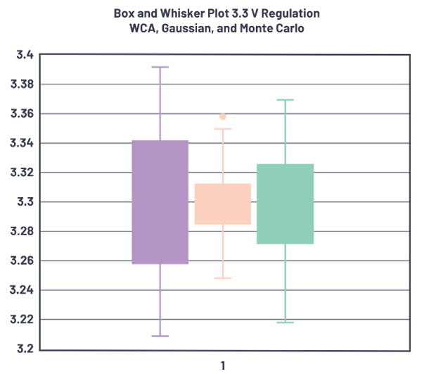
Table 4 and Figure 13 compare the tolerance analysis results. In this example, WCA predicts the largest max deviation, and the simulation based on a Gaussian distribution predicts the smallest. This is illustrated in Figure 13 in a box and whisker plot—the solid box represents the 1-sigma limit, while the whisker represents the minimum and maximum values.
Table 4. Voltage Regulation Statistical Summary for Three Tolerance Analysis Methods
| WCA | Gaussian | Monte Carlo | |
| Average | 3.30013 | 3.29944 | 3.29844 |
| Minimum | 3.21051 | 3.24899 | 3.21955 |
| Maximum | 3.39153 | 3.35720 | 3.36922 |
| Standard Deviation | 0.04684 | 0.01931 | 0.03293 |
| Error Positive | 1.02774 | 1.01733 | 1.02098 |
| Error Positive | 0.97288 | 0.98454 | 0.97562 |
Summary Using a simplified DC-to-DC converter model, three variables have been analyzed, two feedback resistors and the internal voltage reference were used to model voltage setpoint regulation. Using statistical analysis, the resulting voltage setpoint distribution is presented. The results are graphically plotted. This is compared to a worst-case calculation. The resulting data illustrates worst-case limits are statistically improbable.